
Code
%pip install torch gpytorch matplotlib seaborn numpy pandas

import torch
import gpytorch
from matplotlib import pyplot as plt
import numpy as np
import seaborn as sns
import pandas as pdIn my previous post on GPs, we discussed the basics of GPs and their applications in regression tasks. Here, we extend the discussion to multi-task GPs, highlighting their benefits and practical implementations. We will provide an intuitive explanation of the concepts and showcase code examples using GPyTorch. Let’s dive in!
Gaussian processes are a powerful tool for regression and classification tasks, offering a non-parametric way to define distributions over functions. When dealing with multiple related outputs, a multi-task GP can model the dependencies between these tasks, leading to better generalization and predictions.
Mathematically, a Gaussian process is defined as a collection of random variables, any finite number of which have a joint Gaussian distribution. For a set of input points \(X\), the corresponding output values \(f(X)\) are jointly Gaussian:
\[ f(X) \sim \mathcal{N}(m(X), k(X, X)) \]
where \(m(X)\) is the mean function and \(k(X, X)\) is the covariance matrix.
In a multitask setting, we aim to model the function \(f: \mathcal{X} \to \mathbb{R}^T\), so that we have \(T\) outputs, or tasks, \(\{f_t(X)\}_{t=1}^T\). This means that the mean function is \(m: \mathcal{X} \to \mathbb{R}^T\) and the kernel function is \(k: \mathcal{X} \times \mathcal{X} \to \mathbb{R}^{T \times T}\). How can we model the correlations between these tasks?
A simple independent multioutput GP models each task independently, without considering any correlations between tasks. In this setup, each task has its own GP with its own mean and covariance functions. Mathematically, this can be expressed as:
\[ f_i(X) \sim \mathcal{N}(m_i(X), k_i(X, X)) \qquad i = 1, \ldots, T, \]
leading to a block-diagonal covariance matrix \(k(x, x) = \text{diag}(k_1(x, x), \ldots, k_T(x, x))\). This approach does not leverage any shared information between tasks, which can lead to suboptimal performance, especially when there is limited data for some tasks.
The ICM approach generalizes the independent multioutput GP by introducing a coregionalization matrix \(B\) that models the correlations between tasks. Specifically, the covariance function in the ICM approach is defined as:
\[ k(x, x') = k_{\text{input}}(x, x') B, \]
where \(k_{\text{input}}\) is a covariance function defined over the input space (e.g. squared exponential kernel), and \(B \in \mathbb{R}^{T \times T}\) is the coregionalization matrix capturing the task-specific covariances. The matrix \(B\) is typically parameterized as \(B = W W^\mathsf{T}\), with \(W \in \mathbb{R}^{T \times r}\) and \(r\) being the rank of the coregionalization matrix. This ensures the kernel is positive semi-definite.
The ICM approach can learn the shared structure between tasks. Indeed, the Pearson correlation coefficient between tasks can be expressed as:
\[ \rho_{ij} = \frac{B[i, j]}{\sqrt{B[i, i] B[j, j]}}. \]
Another common approach is the LMC model, which extends the ICM by allowing for a wider variety of input kernels. In the LMC model, the covariance function is defined as:
\[ k(x, x') = \sum_{q=1}^Q k_{\text{input}}^{(q)}(x, x') B_q, \]
where \(Q\) is the number of base kernels, \(k_{\text{input}}^{(q)}\) are the base kernels, and \(B_q\) are the coregionalization matrices for each base kernel. This model can capture even more complex correlations between tasks by combining multiple base kernels. We can recover the ICM model by setting \(Q=1\).
In multi-task GPs, we have to consider a multi-output likelihood function that models the noise for each task. The standard likelihood function is typically a multidimensional Gaussian likelihood, which can be expressed as:
\[ y = f(x) + \epsilon, \qquad \epsilon \sim \mathcal{N}_T(0, \Sigma), \]
where \(y\) is the observed output, \(f(x)\) is the latent function, and \(\Sigma\) is the noise covariance matrix. The flexibility is on the choice of the noise covariance matrix, which can be diagonal \(\Sigma = \text{diag}(\sigma_1^2, \ldots, \sigma_T^2)\) (independent noise for each task) or full (correlated noise across tasks). The latter is usually represented as \(\Sigma = L L^\mathsf{T}\), where \(L \in \mathbb{R}^{T \times r}\) and \(r\) is the rank of the noise covariance matrix. This allows for capturing correlations between the noise terms of different tasks.
The final covariance matrix with noise is then given by:
\[ K_n = K + \mathbf{I} \otimes \Sigma, \]
where \(K\) is the covariance matrix without noise, \(\mathbf{I}\) is the identity matrix, and \(\otimes\) denotes the Kronecker product. The noise term is added to the diagonal blocks of the covariance matrix.
GPyTorchLet’s walk through an example of implementing a multitask GP using GPyTorch with the ICM kernel. First of all, we need to install the required packages, including Torch, GPyTorch, matplotlib, and seaborn, numpy.
%pip install torch gpytorch matplotlib seaborn numpy pandas
import torch
import gpytorch
from matplotlib import pyplot as plt
import numpy as np
import seaborn as sns
import pandas as pdAfterward, we can define the multitask GP model. We use an ICM kernel (with rank \(r=1\)) to capture correlations between tasks. We generate synthetic noisy training data for two tasks (sine and a shifted sine), so to have correlated outputs. The noise covariance matrix is
\[ \Sigma = \begin{bmatrix} \sigma_1^2 & \rho \sigma_1 \sigma_2 \\ \rho \sigma_1 \sigma_2 & \sigma_2^2 \end{bmatrix}, \]
where \(\sigma_1^2 = \sigma_2^2 = 0.1^2\) and \(\rho = 0.3\).
Lastly, we train the model and evaluate its performance by plotting the mean predictions and confidence intervals for each task.
# Define the kernel with coregionalization
class MultitaskGPModel(gpytorch.models.ExactGP):
    def __init__(self, train_x, train_y, likelihood, num_tasks):
        super(MultitaskGPModel, self).__init__(train_x, train_y, likelihood)
        self.mean_module = gpytorch.means.MultitaskMean(
            gpytorch.means.ConstantMean(), num_tasks=num_tasks
        )
        self.covar_module = gpytorch.kernels.MultitaskKernel(
            gpytorch.kernels.RBFKernel(), num_tasks=num_tasks, rank=1
        )

    def forward(self, x):
        mean_x = self.mean_module(x)
        covar_x = self.covar_module(x)
        return gpytorch.distributions.MultitaskMultivariateNormal(mean_x, covar_x)

# Training data
f1 = lambda x:  torch.sin(x * (2 * torch.pi))
f2 = lambda x: torch.sin((x - 0.1) * (2 * torch.pi))
train_x = torch.linspace(0, 1, 10)
train_y = torch.stack([
    f1(train_x),
    f2(train_x)
]).T
# Define the noise covariance matrix with correlation = 0.3
sigma2 = 0.1**2
Sigma = torch.tensor([[sigma2, 0.3 * sigma2], [0.3 * sigma2, sigma2]])
# Add noise to the training data
train_y += torch.tensor(np.random.multivariate_normal(mean=[0,0], cov=Sigma, size=len(train_x)))

# Model and likelihood
num_tasks = 2
likelihood = gpytorch.likelihoods.MultitaskGaussianLikelihood(num_tasks=num_tasks, rank=1)
model = MultitaskGPModel(train_x, train_y, likelihood, num_tasks)

# Training the model
model.train()
likelihood.train()

optimizer = torch.optim.Adam(model.parameters(), lr=0.1)

mll = gpytorch.mlls.ExactMarginalLogLikelihood(likelihood, model)

scheduler = torch.optim.lr_scheduler.StepLR(optimizer, step_size=50, gamma=0.5)

num_iter = 500
for i in range(num_iter):
    optimizer.zero_grad()
    output = model(train_x)
    loss = -mll(output, train_y)
    loss.backward()
    optimizer.step()
    scheduler.step()

# Evaluation
model.eval()
likelihood.eval()

test_x = torch.linspace(0, 1, 100)

with torch.no_grad(), gpytorch.settings.fast_pred_var():
    pred_multi = likelihood(model(test_x))

# Plot predictions
fig, ax = plt.subplots()

colors = ['blue', 'red']
for i in range(num_tasks):
    ax.plot(test_x, pred_multi.mean[:, i], label=f'Mean prediction (Task {i+1})', color=colors[i])
    ax.plot(test_x, [f1(test_x), f2(test_x)][i], linestyle='--', label=f'True function (Task {i+1})')
    lower = pred_multi.confidence_region()[0][:, i].detach().numpy()
    upper = pred_multi.confidence_region()[1][:, i].detach().numpy()
    ax.fill_between(
        test_x,
        lower,
        upper,
        alpha=0.2,
        label=f'Confidence interval (Task {i+1})',
        color=colors[i]
    )

ax.scatter(train_x, train_y[:, 0], color='black', label=f'Training data (Task 1)')
ax.scatter(train_x, train_y[:, 1], color='gray', label=f'Training data (Task 2)')

ax.set_title('Multitask GP with ICM')
ax.legend(loc='lower center', bbox_to_anchor=(0.5, -0.2),
          ncol=3, fancybox=True)
Using GPyTorch, the ICM model is straightforward to implement by using the MultitaskMean, MultitaskKernel, and MultitaskGaussianLikelihood classes. These take care of the multitask structure, the noise and coregionalization matrices, allowing us to focus on the model definition and training.
Regarding the training loop, it works similarly to standard GPs, with the negative marginal log-likelihood as the loss function, and an optimizer to update the model parameters. A scheduler has been added to reduce the learning rate during training, which can help stabilize the optimization process.
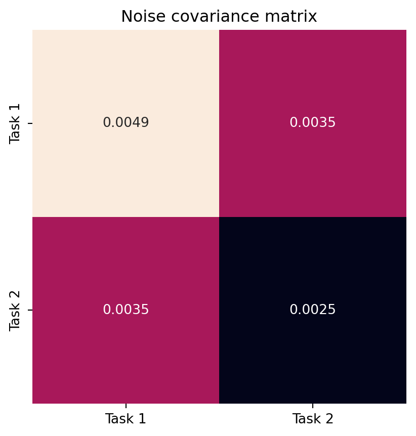
Figure 2 show the coregionalization matrix \(B\) learned by the model, and the noise covariance matrix \(\Sigma\). The former captures the correlations between the tasks. As we can see, the off-diagonal elements of \(B\) are positive. The latter represents the noise levels for each task. Notice that the model has properly learned the noise correlation.
W = model.covar_module.task_covar_module.covar_factor
B = W @ W.T

fig, ax = plt.subplots()
sns.heatmap(B.detach().numpy(), annot=True, ax=ax, cbar=False, square=True)
ax.set_xticklabels(['Task 1', 'Task 2'])
ax.set_yticklabels(['Task 1', 'Task 2'])
ax.set_title('Coregionalization matrix B')
fig.show()


L = model.likelihood.task_noise_covar_factor.detach().numpy()
Sigma = L @ L.T

fig, ax = plt.subplots()
sns.heatmap(Sigma, annot=True, ax=ax, cbar=False, square=True)
ax.set_xticklabels(['Task 1', 'Task 2'])
ax.set_yticklabels(['Task 1', 'Task 2'])
ax.set_title('Noise covariance matrix')
fig.show()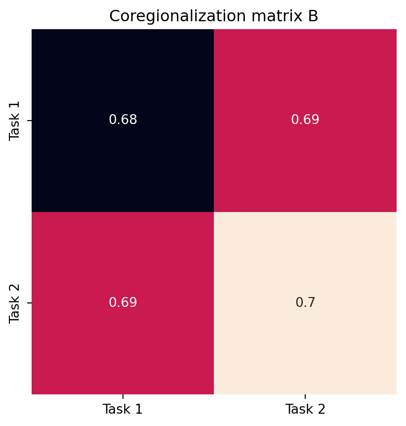
To highlight the advantages of modeling correlated outputs using the ICM approach, let’s compare it with a model that treats each task independently, ignoring any potential correlations between tasks. We can define a separate GP for each task, train them, and evaluate their performance on the test data.
class IndependentGPModel(gpytorch.models.ExactGP):
    def __init__(self, train_x, train_y, likelihood):
        super(IndependentGPModel, self).__init__(train_x, train_y, likelihood)
        self.mean_module = gpytorch.means.ConstantMean()
        self.covar_module = gpytorch.kernels.ScaleKernel(gpytorch.kernels.RBFKernel())

    def forward(self, x):
        mean_x = self.mean_module(x)
        covar_x = self.covar_module(x)
        return gpytorch.distributions.MultivariateNormal(mean_x, covar_x)

# Create models and likelihoods for each task
likelihoods = [gpytorch.likelihoods.GaussianLikelihood() for _ in range(num_tasks)]
models = [IndependentGPModel(train_x, train_y[:, i], likelihoods[i]) for i in range(num_tasks)]

# Training the independent models
for i, (model, likelihood) in enumerate(zip(models, likelihoods)):
    model.train()
    likelihood.train()
    optimizer = torch.optim.Adam(model.parameters(), lr=0.1)
    mll = gpytorch.mlls.ExactMarginalLogLikelihood(likelihood, model)
    scheduler = torch.optim.lr_scheduler.StepLR(optimizer, step_size=50, gamma=0.5)

    for _ in range(num_iter):
        optimizer.zero_grad()
        output = model(train_x)
        loss = -mll(output, train_y[:, i])
        loss.backward()
        optimizer.step()
        scheduler.step()

# Evaluation
for model, likelihood in zip(models, likelihoods):
    model.eval()
    likelihood.eval()

with torch.no_grad(), gpytorch.settings.fast_pred_var():
    pred_inde = [likelihood(model(test_x)) for model, likelihood in zip(models, likelihoods)]

# Plot predictions
fig, ax = plt.subplots()

for i in range(num_tasks):
    ax.plot(test_x, pred_inde[i].mean, label=f'Mean prediction (Task {i+1})', color=colors[i])
    ax.plot(test_x, [f1(test_x), f2(test_x)][i], linestyle='--', label=f'True function (Task {i+1})')
    lower = pred_inde[i].confidence_region()[0]
    upper = pred_inde[i].confidence_region()[1]
    ax.fill_between(
        test_x,
        lower,
        upper,
        alpha=0.2,
        label=f'Confidence interval (Task {i+1})',
        color=colors[i]
    )

ax.scatter(train_x, train_y[:, 0], color='black', label='Training data (Task 1)')
ax.scatter(train_x, train_y[:, 1], color='gray', label='Training data (Task 2)')

ax.set_title('Independent GPs')
ax.legend(loc='lower center', bbox_to_anchor=(0.5, -0.2),
          ncol=3, fancybox=True)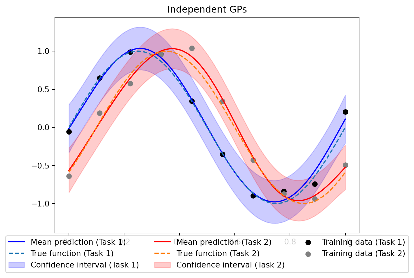
In terms of performance, we can compare the mean squared error (MSE) of the predictions on the test data for the multitask GP with ICM and the independent GPs.
mean_multi = pred_multi.mean.numpy()
mean_inde = np.stack([pred.mean.numpy() for pred in pred_inde]).T

test_y = torch.stack([f1(test_x), f2(test_x)]).T.numpy()
MSE_multi = np.mean((mean_multi - test_y) ** 2)
MSE_inde = np.mean((mean_inde - test_y) ** 2)

df = pd.DataFrame({
    'Model': ['ICM', 'Independent'],
    'MSE': [MSE_multi, MSE_inde]
  })
df| Model | MSE | |
|---|---|---|
| 0 | ICM | 0.002097 |
| 1 | Independent | 0.002626 |
The results show that ICM slightly outperforms the independent GPs in terms of MSE, thanks to the shared structure learned by the coregionalization matrix. In practice, the improvement can be more significant when dealing with more complex tasks or limited data. Indeed, in the independent scenario, each GP learns from a smaller dataset of 10 points, potentially leading to overfitting or suboptimal generalization. On the other hand, the multitask GP with ICM uses all the 20 points to learn the squared exponential kernel parameters. This shared information helps to improve the predictions for both tasks.