Welcome to the first installment of our series on deep kernel learning. In this post, we’ll delve into Gaussian processes (GPs) and their application as regressors. We’ll start by exploring what GPs are and why they are powerful tools for regression tasks. In subsequent posts, we’ll build on this foundation to discuss multi-task Gaussian processes and how they can be combined with neural networks to create deep kernel models.
Gaussian processes
To understand Gaussian processes fully, it’s important to briefly mention the Kolmogorov extension theorem. This theorem guarantees the existence of a stochastic process, i.e., a collection of random variables \(\{Y_x\}_{x \in \mathcal{X}}, Y_x \in \mathbb{R}\), that satisfies a specified finite-dimensional distribution. For instance, it ensures that we can define a Gaussian process by specyfing that any finite set of random variables has a multivariate Gaussian distribution, without worrying about the infinite-dimensional nature of the process. Observe that, in a similar matter, we could define a t-student process, by imposing that finite-dimensional distributions are t-student.
Therefore, similar to a multivariate Gaussian distribution, a Gaussian process \(f\) is defined by its mean function \(m(\cdot) : \mathcal{X} \to \mathbb{R}\) and covariance function \(k(\cdot, \cdot) : \mathcal{X} \times \mathcal{X} \to \mathbb{R}\):
\[
f \sim GP(m, k),
\]
and it can be interpreted as an infinite-dimensional generalization of a multivariate Gaussian distribution.
In a regression setting, we could use \(f\) as a surrogate model of a function \(g: \mathcal{X} \to \mathbb{R}\), where \(\mathcal{X}\) is the input space. Suppose you have a set of input points \(X = \{x_1, x_2, \ldots, x_n\}\), with observations \(Y = \{y_1 = g(x_1), y_2 = g(x_2), \ldots, y_n = g(x_n)\}\), the joint distribution of the observed outputs \(Y\), assuming a GP prior, is given by:
where \(\mathbf{m}\) is the vector of mean function values and \(\mathbf{K}\) is the covariance matrix of the function values at the input points. This approach allows us to make predictions at new input points \(x_*\) by conditioning on the observed data, providing not only point estimates but also uncertainty estimates.
Making predictions
To make a prediction \(y_* = g(x_*)\) at new input point, we use the joint distribution of the observed outputs \(Y\) and the function values at \(x_*\), which is given by:
where \(k(x_*, X)\) is vector of covariances between the new input point \(x_*\) and the observed data points \(X\). The conditional distribution of \(y_*\) given \(Y\) is then Gaussian with mean and covariance:
Therefore, given the observed data, we can estimate the function value at a new input point \(x_*\) as \(\mu(x_*)\) and quantify the uncertainty in the prediction as \(s^2(x_*)\). This is a key advantage of GPs, which can be important in decision-making processes.
Interactive visualizations
Let’s explore some interactive plots to better understand how the kernel functions influence the Gaussian process model. Indeed, the choice of the kernel function is crucial in defining the prior over functions, as it determines the smoothness and periodicity of the functions that the GP can model. Therefore, they play a fundamental role in the model’s flexibility and generalization capabilities, and they can be tailored to the specific characteristics of the data at hand. On the other hand, the mean function is usually set constant, as the kernel is flexible enough.
Squared exponential kernel
The squared exponential kernel (also known as the RBF kernel) is defined as:
where \(\sigma^2\) is the variance and \(l\) is the length scale. Below is an interactive plot that shows how the squared exponential kernel depends on the lengthscale and variance. Notice that with a small length scale, the function is more wiggly. Instead, with a large length scale it is smoother, as the kernel function decays more slowly with distance (i.e., the correlation between faraway points is higher, and they are more similar to each other). Instead, the variance controls the amplitude of the function, with higher values leading to more variability.
#| standalone: true
#| viewerHeight: 475

import numpy as np
import matplotlib.pyplot as plt
from scipy.stats import multivariate_normal
from shiny import App, render, ui


# Define the kernel function
def exponential_quadratic_kernel(x1, x2, l=1.0, sigma2=1.0):
    """Computes the exponential quadratic kernel (squared exponential kernel)."""
    sqdist = np.sum(x1**2, 1).reshape(-1, 1) + np.sum(x2**2, 1) - 2 * np.dot(x1, x2.T)
    return sigma2 * np.exp(-0.5 / l**2 * sqdist)

# Define the input space
X = np.linspace(-4, 4, 100).reshape(-1, 1)

def plot_kernel_and_samples(l, sigma2):
    # Compute the kernel matrix
    K = exponential_quadratic_kernel(X, X, l=l, sigma2=sigma2)

    # Create the plot
    fig, ax = plt.subplots(2, 1, figsize=(18, 6), sharex=True)

    # Plot the kernel
    ax[0].plot(X, exponential_quadratic_kernel(X, np.zeros((1,1)), l=l, sigma2=sigma2))
    ax[0].set_title(f"Squared exponential kernel function")

    # Sample 5 functions from the Gaussian process defined by the kernel
    mean = np.zeros(100)
    cov = K
    samples = multivariate_normal.rvs(mean, cov, 5)

    # Plot the samples
    for i in range(5):
        ax[1].plot(X, samples[i])
    ax[1].set_title("Samples from the GP")
    ax[1].set_xlabel("x")

    plt.tight_layout()
    return fig

app_ui = ui.page_fluid(
    ui.layout_sidebar(
        ui.panel_sidebar(
            ui.input_slider("length_scale", "Length Scale (l):", min=0.1, max=5.0, value=1.0, step=0.1),
            ui.input_slider("variance", "Variance (σ²):", min=0.1, max=5.0, value=1.0, step=0.1)
        ),
        ui.panel_main(
            ui.output_plot("kernelPlot")
        )
    )
)

def server(input, output, session):
    @output
    @render.plot
    def kernelPlot():
        l = input.length_scale()
        sigma2 = input.variance()
        fig = plot_kernel_and_samples(l, sigma2)
        return fig

app = App(app_ui, server)
where \(\nu\) controls the smoothness of the function, \(l\) is the length scale, \(\sigma^2\) is the variance, and \(K_{\nu}\) is the modified Bessel function. The former two parameters have the same effect as in the squared exponential kernel, while \(\nu\) controls the smoothness of the function. Indeed, we have that the samples generated have smoothness \(\lceil \nu \rceil - 1\), and for \(\nu \to \infty\), the Matérn kernel converges to the squared exponential kernel, leading to infinitely smooth functions.
#| standalone: true
#| viewerHeight: 475

import numpy as np
import matplotlib.pyplot as plt
from scipy.stats import multivariate_normal
from shiny import App, render, ui
from scipy.special import kv, gamma
from scipy.spatial.distance import cdist


# Define the kernel function
def matern_kernel(x1, x2, l=1.0, sigma2=1.0, nu=1.5):
    """Computes the Matérn kernel."""
    D = cdist(x1, x2, 'euclidean')
    const = (2**(1-nu))/gamma(nu)
    K = const * (np.sqrt(2*nu)*D/l)**nu * kv(nu, np.sqrt(2*nu)*D/l)
    # Replace NaN values with 1 for x == x'
    K[np.isnan(K)] = 1
    K *= sigma2
    return K

# Define the input space
X = np.linspace(-4, 4, 100).reshape(-1, 1)

def plot_kernel_and_samples(l, sigma2, nu):
    # Compute the kernel matrix
    K = matern_kernel(X, X, l=l, sigma2=sigma2, nu=nu)

    # Create the plot
    fig, ax = plt.subplots(2, 1, figsize=(18, 6), sharex=True)

    # Plot the kernel
    ax[0].plot(X, matern_kernel(X, np.zeros((1, 1)), l=l, sigma2=sigma2, nu=nu))
    ax[0].set_title(f"Matern kernel function")

    # Sample 5 functions from the Gaussian process defined by the kernel
    mean = np.zeros(100)
    cov = K
    samples = multivariate_normal.rvs(mean, cov, 5)

    # Plot the samples
    for i in range(5):
        ax[1].plot(X, samples[i])
    ax[1].set_title("Samples from the GP")
    ax[1].set_xlabel("x")

    plt.tight_layout()
    return fig

app_ui = ui.page_fluid(
    ui.layout_sidebar(
        ui.panel_sidebar(
            ui.input_slider("length_scale", "Length Scale (l):", min=0.1, max=5.0, value=1.0, step=0.1),
            ui.input_slider("variance", "Variance (σ²):", min=0.1, max=5.0, value=1.0, step=0.1),
            ui.input_slider("smoothness_param", "Smoothness param (v):", min=1.5, max=5.0, value=1.5, step=0.5)
        ),
        ui.panel_main(
            ui.output_plot("kernelPlot")
        )
    )
)

def server(input, output, session):
    @output
    @render.plot
    def kernelPlot():
        l = input.length_scale()
        sigma2 = input.variance()
        nu = input.smoothness_param()
        fig = plot_kernel_and_samples(l, sigma2, nu)
        return fig

app = App(app_ui, server)
Noisy observations
Noise and measurement error are inevitable in real-world data, which can significantly impact the performance and reliability of predictive models. As a result, it is essential to take noise into account when modeling data with GP. We can represent noisy observations as:
\[
y = g(x) + \epsilon
\]
where \(\epsilon\) is a random variable representing the noise. Usually, we assume that \(\epsilon \sim \mathcal{N}(0, \sigma_n^2)\), where \(\sigma_n^2\) is the variance of the noise. In this way, it can be easily incorporated into the GP by adding a diagonal noise term to the kernel matrix:
where \(\mathbf{K}\) is the kernel matrix computed on the training data and \(\mathbf{I}\) is the identity matrix.
Below is an interactive plot that demonstrates how noise influences the GP model. The plot shows the noisy training data (black points) of the true function \(g(x) = \sin(x)\), the red dashed line. The plot also shows the GP mean prediction (blue line) for the squared exponential and Matérn kernels, along with the 95% confidence intervals. For \(\sigma_n^2 = 0\), the model perfectly interpolates the training data. For higher noise levels, the model becomes less certain about the observations, leading to a non-interpolating behavior, and the confidence intervals widen.
#| standalone: true
#| viewerHeight: 475

import numpy as np
import matplotlib.pyplot as plt
from scipy.stats import multivariate_normal
from shiny import App, render, ui
from scipy.spatial.distance import cdist
from scipy.special import kv, gamma

# Define the kernel functions
def exponential_quadratic_kernel(x1, x2, l=1.0, sigma2=1.0):
    """Computes the exponential quadratic kernel (squared exponential kernel)."""
    sqdist = np.sum(x1**2, 1).reshape(-1, 1) + np.sum(x2**2, 1) - 2 * np.dot(x1, x2.T)
    return sigma2 * np.exp(-0.5 / l**2 * sqdist)

def matern_kernel(x1, x2, l=1.0, sigma2=1.0, nu=1.5):
    """Computes the Matérn kernel."""
    D = cdist(x1, x2, 'euclidean')
    const = (2**(1-nu))/gamma(nu)
    K = sigma2 * const * (np.sqrt(2*nu)*D/l)**nu * kv(nu, np.sqrt(2*nu)*D/l)
    # Replace NaN values with 1 for x == x'
    K[np.isnan(K)] = 1
    return K

# Define the input space
X = np.linspace(-4, 4, 100).reshape(-1, 1)

def plot_kernels_and_samples(noise_level):
    # Generate training data with noise
    X_train = np.array([-3, -2, -1, 1, 3.5]).reshape(-1, 1)
    y_train = np.sin(X_train) + noise_level * np.random.randn(X_train.shape[0], 1).reshape(-1,1)

    # Compute the kernel matrices for training data
    K_train_exp = exponential_quadratic_kernel(X_train, X_train) + noise_level**2 * np.eye(len(X_train))
    K_s_exp = exponential_quadratic_kernel(X_train, X)
    K_ss_exp = exponential_quadratic_kernel(X, X)

    K_train_matern = matern_kernel(X_train, X_train) + noise_level**2 * np.eye(len(X_train))
    K_s_matern = matern_kernel(X_train, X)
    K_ss_matern = matern_kernel(X, X)

    # Compute the mean and covariance of the posterior distribution for exponential kernel
    K_train_inv_exp = np.linalg.inv(K_train_exp)
    mu_s_exp = (K_s_exp.T.dot(K_train_inv_exp).dot(y_train)).reshape(-1)
    cov_s_exp = K_ss_exp - K_s_exp.T.dot(K_train_inv_exp).dot(K_s_exp)

    # Compute the mean and covariance of the posterior distribution for Matérn kernel
    K_train_inv_matern = np.linalg.inv(K_train_matern)
    mu_s_matern = (K_s_matern.T.dot(K_train_inv_matern).dot(y_train)).reshape(-1)
    cov_s_matern = K_ss_matern - K_s_matern.T.dot(K_train_inv_matern).dot(K_s_matern)

    # Sample 5 functions from the posterior distribution for both kernels
    samples_exp = multivariate_normal.rvs(mu_s_exp, cov_s_exp, 5)
    samples_matern = multivariate_normal.rvs(mu_s_matern, cov_s_matern, 5)

    # Create the plot
    fig, ax = plt.subplots(2, 1, figsize=(18, 6), sharex=True)

    # Plot the training data and GP predictions for exponential kernel
    ax[0].scatter(X_train, y_train, color='black', zorder=10, label='Noisy observations')
    ax[0].plot(X, mu_s_exp, color='blue', label='Mean prediction')
    ax[0].plot(X, np.sin(X), color='r', linestyle='--', label='True function')
    ax[0].fill_between(X.ravel(), mu_s_exp - 1.96 * np.sqrt(np.diag(cov_s_exp)), mu_s_exp + 1.96 * np.sqrt(np.diag(cov_s_exp)), color="blue", alpha=0.2, label='Confidence interval')
    # for i in range(5):
    #     ax[0].plot(X, samples_exp[i], alpha=0.5, linestyle='--')
    ax[0].set_title(f"Squared exponential kernel")
    # ax[0].legend()

    # Plot the training data and GP predictions for Matérn kernel
    ax[1].scatter(X_train, y_train, color='black', zorder=10, label='Noisy observations')
    ax[1].plot(X, mu_s_matern, color="blue", label='Mean prediction')
    ax[1].plot(X, np.sin(X), color="r", linestyle='--', label='True function')
    ax[1].fill_between(X.ravel(), mu_s_matern - 1.96 * np.sqrt(np.diag(cov_s_matern)), mu_s_matern + 1.96 * np.sqrt(np.diag(cov_s_matern)), color="blue", alpha=0.2, label='Confidence interval')
    # for i in range(5):
    #     ax[1].plot(X, samples_matern[i], alpha=0.5, linestyle='--')
    ax[1].set_title(f"Matérn kernel")
    # ax[1].legend()
    ax[1].set_xlabel("x")

    plt.tight_layout()
    return fig

app_ui = ui.page_fluid(
    ui.layout_sidebar(
        ui.panel_sidebar(
            ui.input_slider("noise_level", "Noise Level (σ²ₙ):", min=0.0, max=1.0, value=0.0, step=0.01)
        ),
        ui.panel_main(
            ui.output_plot("kernelPlot")
        )
    )
)

def server(input, output, session):
    @output
    @render.plot
    def kernelPlot():
        noise_level = input.noise_level()
        fig = plot_kernels_and_samples(noise_level)
        return fig

app = App(app_ui, server)
Code
In this section, we’ll provide a brief overview of how to implement Gaussian processes in Python using the GPyTorch library. The code snippet below demonstrates how to define a GP model with a squared exponential kernel and train it on synthetic data.
Code
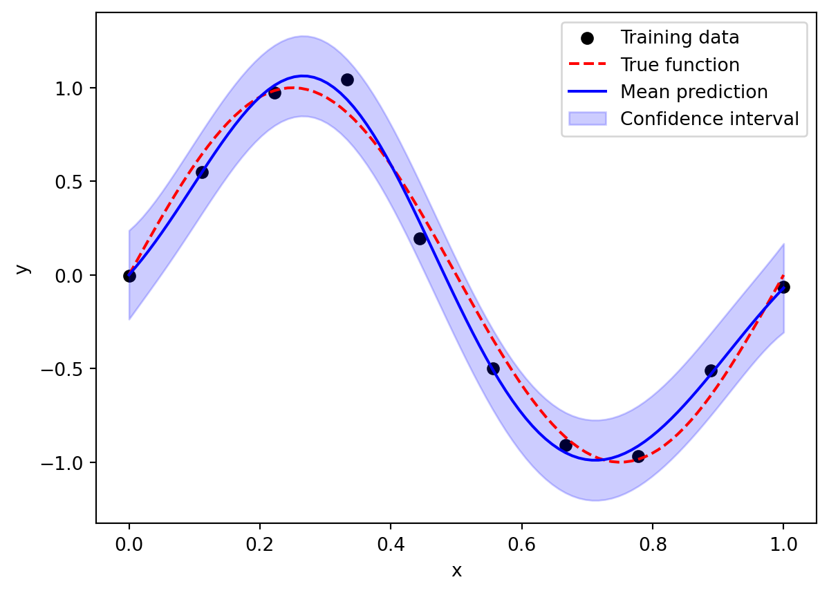
import numpy as npimport matplotlib.pyplot as pltimport torchimport gpytorchfrom gpytorch.kernels import RBFKernel, ScaleKernelfrom gpytorch.means import ConstantMeanfrom gpytorch.likelihoods import GaussianLikelihoodfrom gpytorch.models import ExactGPfrom gpytorch.mlls import ExactMarginalLogLikelihoodfrom gpytorch.distributions import MultivariateNormal# Define the GP modelclass GP(ExactGP):def__init__(self, train_x, train_y, likelihood):super(GP, self).__init__(train_x, train_y, likelihood)self.mean_module = ConstantMean()self.covar_module = ScaleKernel(RBFKernel())def forward(self, x): mean_x =self.mean_module(x) covar_x =self.covar_module(x)return MultivariateNormal(mean_x, covar_x)# Generate synthetic dataf =lambda x: torch.sin(x * (2* np.pi))train_x = torch.linspace(0, 1, 10)train_y = f(train_x) + torch.randn(train_x.size()) *0.1likelihood = GaussianLikelihood()# Initialize the model and likelihoodmodel = GP(train_x, train_y, likelihood)# Training the modelmodel.train()likelihood.train()# Use the adam optimizeroptimizer = torch.optim.Adam(model.parameters(), lr=0.1)# "Loss" for GPs - the marginal log likelihoodmll = ExactMarginalLogLikelihood(likelihood, model)# Training looptraining_iterations =50for i inrange(training_iterations): optimizer.zero_grad() output = model(train_x) loss =-mll(output, train_y) loss.backward() optimizer.step()# Set the model and likelihood into evaluation modemodel.eval()likelihood.eval()# Make predictionstest_x = torch.linspace(0, 1, 100)with torch.no_grad(), gpytorch.settings.fast_pred_var(): observed_pred = likelihood(model(test_x)) mean = observed_pred.mean lower, upper = observed_pred.confidence_region()# Plot the resultsfig, ax = plt.subplots()ax.scatter(train_x, train_y, color='black', label='Training data')ax.plot(test_x, f(test_x), 'r--', label='True function')ax.plot(test_x, mean, 'b', label='Mean prediction')ax.fill_between(test_x, lower, upper, alpha=0.2, color='blue', label='Confidence interval')ax.set_xlabel('x')ax.set_ylabel('y')ax.legend()
The three main components that need to be defined are the mean function, the kernel function, and the likelihood function (which models the noise in the data). Observe that the base kernel is the RBFKernel, which corresponds to the squared exponential kernel, and it is wrapped by the ScaleKernel to allow for the scaling of the kernel through the variance parameter \(\sigma^2\). The ExactMarginalLogLikelihood object is used to compute the marginal log likelihood, which is the negative loss function for training the GP model. Indeed, the GP model parameters are optimized by maximizing the marginal log likelihood of the observed data, which is given by
where \(\theta\) are the model parameters, comprising the mean, kernel, and likelihood parameters. Computaionally speaking, the inversion of the kernel matrix \(\mathbf{K}_n\) is the most expensive operation, with a complexity of \(\mathcal{O}(n^3)\), where \(n\) is the number of training points. Therefore, for very large datasets, approximate inference methods, inducing points, or sparse GPs should be used to reduce the computational burden.
Lastly, observe that the ExactGP class is the standard GP for Gaussian likelihoods, where the exact marginal log likelihood can be computed in closed form. However, GPyTorch also provides different likelihoods, such as student-t likelihoods (which is more stable if outliers are present) and more. In these cases, the must class ApproximateGP should be used, which allows for approximate inference methods like variational inference. Regarding the loss function, the ExactMarginalLogLikelihood should be replaced by the VariationalELBO object, or other appropriate loss functions for approximate inference.
Applications
Bayesian hyperparameter tuning
Hyperparameter tuning is a critical yet challenging aspect of training neural networks. Finding the optimal combination of hyperparameters, such as learning rate, batch size, number of layers, and units per layer, can significantly enhance a model’s performance. Traditional methods like grid search and random search often prove to be inefficient and computationally expensive. This is where Bayesian optimization, powered by GPs, comes into play, offering a smarter approach to hyperparameter tuning.
Unlike exhaustive search methods, Bayesian optimization is more sample-efficient, meaning it can find optimal hyperparameters with fewer iterations. It works by
modeling the objective function (e.g., validation loss) as a GP in the hyperparameter space.
using an acquisition function to decide where to sample next. The acquisition function balances exploration (sampling in unexplored regions) and exploitation (sampling in regions with low loss) to guide the search towards the global optimum.
Surrogate optimization
GPs are also used in surrogate optimization, where the objective function is expensive to evaluate, and we aim to find the global optimum with as few evaluations as possible. By modeling the objective function as a GP, we can make informed decisions about where to sample next, focusing on regions that are likely to contain the global optimum. This can significantly reduce the number of evaluations needed to find the best solution.
Time series forecasting
GPs are also widely used in time series forecasting due to their flexibility and ability to model complex patterns in the data. By treating time series data as a function of time, Gaussian processes can capture the underlying dynamics and dependencies in the series. They can provide not only point estimates but also probabilistic forecasts, including prediction intervals that quantify uncertainty.